Pruning deep neural networks to make them fast and small
The PyTorch implementation of [1611.06440 Pruning Convolutional Neural Networks for Resource Efficient Inference].
TL;DR: By using pruning a VGG-16 based Dogs-vs-Cats classifier is made x3 faster and x4 smaller.
Pruning neural networks is an old idea going back to 1990 (with Yan Lecun’s optimal brain damage work) and before. The idea is that among the many parameters in the network, some are redundant and don’t contribute a lot to the output.
If you could rank the neurons in the network according to how much they contribute, you could then remove the low ranking neurons from the network, resulting in a smaller and faster network.
Getting faster/smaller networks is important for running these deep learning networks on mobile devices.
The ranking can be done according to the L1/L2 mean of neuron weights, their mean activations, the number of times a neuron wasn’t zero on some validation set, and other creative methods . After the pruning, the accuracy will drop (hopefully not too much if the ranking clever), and the network is usually trained more to recover.
If we prune too much at once, the network might be damaged so much it won’t be able to recover.
So in practice this is an iterative process – often called ‘Iterative Pruning’: Prune / Train / Repeat.
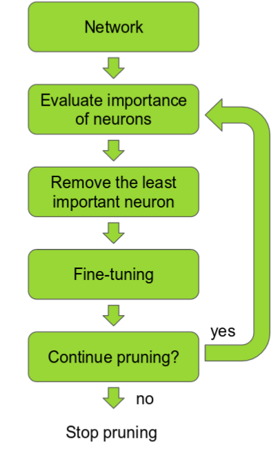
The image is taken from [1611.06440 Pruning Convolutional Neural Networks for Resource Efficient Inference]
Sounds good, why isn’t this more popular?
There are a lot of papers about pruning, but I’ve never encountered pruning used in real life deep learning projects.
Which is surprising considering all the effort on running deep learning on mobile devices. I guess the reason is a combination of:
- The ranking methods weren’t good enough until now, resulting in too big of an accuracy drop.
- It’s a pain to implement.
- Those who do use pruning, keep it for themselves as a secret sauce advantage.
So, I decided to implement pruning myself and see if I could get good results with it.
In this post we will go over a few pruning methods, and then dive into the implementation details of one of the recent methods.
We will fine tune a VGG network to classify cats/dogs on the Kaggle Dogs vs Cats dataset, which represents a kind of transfer learning that I think is very common in practice.
Then we will prune the network and speed it up by a factor of almost x3, and reduce the size by a factor of almost x4!
Pruning for speed vs Pruning for a small model
In VGG16 90% of the weights are in the fully connected layers, but those account for 1% of the total floating point operations.
Up until recently most of the works focused on pruning the fully connected layers. By pruning those, the model size can be dramatically reduced.
We will focus here on pruning entire filters in convolutional layers.
But this has a cool side affect of also reducing memory. As observed in the [1611.06440 Pruning Convolutional Neural Networks for Resource Efficient Inference] paper, the deeper the layer, the more it will get pruned.
This means the last convolutional layer will get pruned a lot, and a lot of neurons from the fully connected layer following it will also be discarded!
When pruning the convolutional filters, another option would be to reduce the weights in each filter, or remove a specific dimension of a single kernel. You can end up with filters that are sparse, but it’s not trivial the get a computational speed up. Recent works advocate “Structured sparsity” where entire filters are pruned instead.
One important thing several of these papers show, is that by training and then pruning a larger network, especially in the case of transfer learning, they get results that are much better than training a smaller network from scratch.
Lets now briefly review a few methods.
[1608.08710 Pruning filters for effecient convnets]
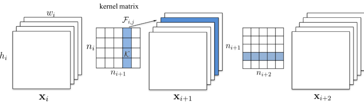
In this work they advocate pruning entire convolutional filters. Pruning a filter with index k affects the layer it resides in, and the following layer. All the input channels at index k, in the following layer, will have to removed, since they won’t exist any more after the pruning.

The image is from [1608.08710 Pruning filters for effecient convnets]
In case the following layer is a fully connected layer, and the size of the feature map of that channel would be MxN, then MxN neurons be removed from the fully connected layer.
The neuron ranking in this work is fairly simple. It’s the L1 norm of the weights of each filter.
At each pruning iteration they rank all the filters, prune the m lowest ranking filters globally among all the layers, retrain and repeat.
[1512.08571 Structured Pruning of Deep Convolutional Neural Networks]
This work seems similar, but the ranking is much more complex. They keep a set of N particle filters, which represent N convolutional filters to be pruned.
Each particle is assigned a score based on the network accuracy on a validation set, when the filter represented by the particle was not masked out. Then based on the new score, new pruning masks are sampled.
Since running this process is heavy, they used a small validation set for measuring the particle scores.
[1611.06440 Pruning Convolutional Neural Networks for Resource Efficient Inference]
This is a really cool work from Nvidia.
First they state the pruning problem as a combinatorial optimization problem: choose a subset of weights B, such that when pruning them the network cost change will be minimal.
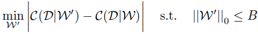
Notice how they used the absolute difference and not just the difference. Using the absolute difference enforces that the pruned network won’t decrease the network performance too much, but it also shouldn’t increase it. In the paper they show this gives better results, presumably because it’s more stable.
Now all ranking methods can be judged by this cost function.
Oracle pruning
VGG16 has 4224 convolutional filters. The “ideal” ranking method would be brute force – prune each filter, and then observe how the cost function changes when running on the training set. Since they are from Nvidia and they have access to a gazillion GPUs they did just that. This is called the oracle ranking – the best possible ranking for minimizing the network cost change. Now to measure the effectiveness of other ranking methods, they compute the spearman correlation with the oracle. Surprise surprise, the ranking method they came up with (described next) correlates most with the oracle.
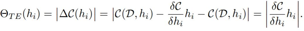
They come up with a new neuron ranking method based on a first order (meaning fast to compute) Taylor expansion of the network cost function.
Pruning a filter h is the same as zeroing it out.
C(W, D) is the average network cost function on the dataset D, when the network weights are set to W. Now we can evaluate C(W, D) as an expansion around C(W, D, h = 0). They should be pretty close, since removing a single filter shouldn’t affect the cost too much.
The ranking of h is then abs(C(W, D, h = 0) – C(W, D)).
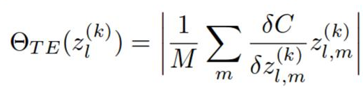
The rankings of each layer are then normalized by the L2 norm of the ranks in that layer. I guess this kind of empiric, and i’m not sure why is this needed, but it greatly effects the quality of the pruning.
This rank is quite intuitive. We could’ve used both the activation, and the gradient, as ranking methods by themselves. If any of them are high, that means they are significant to the output. Multiplying them gives us a way to throw/keep the filter if either the gradients or the activations are very low or high.
This makes me wonder – did they pose the pruning problem as minimizing the difference of the network costs, and then come up with the taylor expansion method, or was it other way around, and the difference of network costs oracle was a way to back up their new method ? 🙂
In the paper their method outperformed other methods in accuracy, too, so it looks like the oracle is a good indicator.
Anyway I think this is a nice method that’s more friendly to code and test, than say, a particle filter, so we will explore this further!
Pruning a Cats vs Dogs classifier using the Taylor criteria ranking
So lets say we have a transfer learning task where we need to create a classifier from a relatively small dataset. Like in this Keras blog post.
Can we use a powerful pre-trained network like VGG for transfer learning, and then prune the network?
If many features learned in VGG16 are about cars, peoples and houses – how much do they contribute to a simple dog/cat classifier ?
This is a kind of a problem that I think is very common.
As a training set we will use 1000 images of cats, and 1000 images of dogs, from the Kaggle Dogs vs Cats data set. As a testing set we will use 400 images of cats, and 400 images of dogs.
First lets show off some statistics.
The accuracy dropped from 98.7% to 97.5%.
The network size reduced from 538 MB to 150 MB.
On a i7 CPU the inference time reduced from 0.78 to 0.277 seconds for a single image, almost a factor x3 reduction!
Step one – train a large network
We will take VGG16, drop the fully connected layers, and add three new fully connected layers. We will freeze the convolutional layers, and retrain only the new fully connected layers. In PyTorch, the new layers look like this:
self.classifier = nn.Sequential(
        nn.Dropout(),
        nn.Linear(25088, 4096),
        nn.ReLU(inplace=True),
        nn.Dropout(),
        nn.Linear(4096, 4096),
        nn.ReLU(inplace=True),
        nn.Linear(4096, 2))
After training for 20 epoches with data augmentation, we get an accuracy of 98.7% on the testing set.
Step two – Rank the filters
To compute the Taylor criteria, we need to perform a Forward+Backward pass on our dataset (or on a smaller part of it if it’s too large. but since we have only 2000 images lets use that).
Now we need to somehow get both the gradients and the activations for convolutional layers. In PyTorch we can register a hook on the gradient computation, so a callback is called when they are ready:
for layer, (name, module) in enumerate(self.model.features._modules.items()):
    x = module(x)
    if isinstance(module, torch.nn.modules.conv.Conv2d):
        x.register_hook(self.compute_rank)
        self.activations.append(x)
        self.activation_to_layer[activation_index] = layer
        activation_index += 1
Now we have the activations in self.activations, and when a gradient is ready, compute_rank will be called:
def compute_rank(self, grad):
    activation_index = len(self.activations) - self.grad_index - 1
    activation = self.activations[activation_index]
    values = \
        torch.sum((activation * grad), dim = 0).\
            sum(dim=2).sum(dim=3)[0, :, 0, 0].data

    # Normalize the rank by the filter dimensions
    values = \
        values / (activation.size(0) * activation.size(2) * activation.size(3))

    if activation_index not in self.filter_ranks:
        self.filter_ranks[activation_index] = \
            torch.FloatTensor(activation.size(1)).zero_().cuda()

    self.filter_ranks[activation_index] += values
    self.grad_index += 1
This did a point wise multiplication of each activation in the batch and it’s gradient, and then for each activation (that is an output of a convolution) we sum in all dimensions except the dimension of the output.
For example, if the batch size was 32, the number of outputs for a specific activation was 256 and the spatial size of that activation was 112×112 such the activation/gradient shapes were 32x256x112x112, then the output will be a 256 sized vector representing the ranks of the 256 filters in this layer.
Now that we have the ranking, we can use a min heap to get the N lowest ranking filters. Unlike in the Nvidia paper where they used N=1 at each iteration, to get results faster we will use N=512! This means that each pruning iteration, we will remove 12% from the original number of the 4224 convolutional filters.
The distribution of the low ranking filters is interesting. Most of the filters pruned are from the deeper layer. Here is a peek of which filters were pruned after the first iteration:
| Layer number | Number of pruned filters pruned |
|---|---|
| Layer 0 | 6 |
| Layer 2 | 1 |
| Layer 5 | 4 |
| Layer 7 | 3 |
| Layer 10 | 23 |
| Layer 12 | 13 |
| Layer 14 | 9 |
| Layer 17 | 51 |
| Layer 19 | 35 |
| Layer 21 | 52 |
| Layer 24 | 68 |
| Layer 26 | 74 |
| Layer 28 | 73 |
Step 3 – Fine tune and repeat
At this stage, we unfreeze all the layers and retrain the network for 10 epoches, which was enough to get good results on this dataset. Then we go back to step 1 with the modified network, and repeat.
This is the real price we pay – that’s 50% of the number of epoches used to train the network, at a single iteration. In this toy dataset we can get away with it since the dataset is small. If you’re doing this for a huge dataset, you better have lots of GPUs.
Summary
I think pruning is an overlooked method that is going to get a lot more attention and use in practice. We showed how we can get nice results on a toy dataset. I think many problems deep learning is used to solve in practice are similar to this one, using transfer learning on a limited dataset, so they can benefit from pruning too.