The 5 Clustering Algorithms Data Scientists Need to Know

By George Seif
Twitter: twitter.com/GeorgeSeif94

Clustering is a Machine Learning technique that involves the grouping of data points. Given a set of data points, we can use a clustering algorithm to classify each data point into a specific group. In theory, data points that are in the same group should have similar properties and/or features, while data points in different groups should have highly dissimilar properties and/or features. Clustering is a method of unsupervised learning and is a common technique for statistical data analysis used in many fields.

In Data Science, we can use clustering analysis to gain some valuable insights from our data by seeing what groups the data points fall into when we apply a clustering algorithm. Today, we’re going to look at 5 popular clustering algorithms that data scientists need to know and their pros and cons!

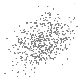
K-Means Clustering

K-Means is probably the most well know clustering algorithm. It’s taught in a lot of introductory data science and machine learning classes. It’s easy to understand and implement in code! Check out the graphic below for an illustration.

K-Means Clustering

1. 1. To begin, we first select a number of classes/groups to use and randomly initialize their respective center points. To figure out the number of classes to use, it’s good to take a quick look at the data and try to identify any distinct groupings. The center points are vectors of the same length as each data point vector and are the “X’s” in the graphic above.
   2. Each data point is classified by computing the distance between that point and each group center, and then classifying the point to be in the group whose center is closest to it.
   3. Based on these classified points, we recompute the group center by taking the mean of all the vectors in the group.
   4. Repeat these steps for a set number of iterations or until the group centers don’t change much between iterations. You can also opt to randomly initialize the group centers a few times, and then select the run that looks like it provided the best results.

K-Means has the advantage that it’s pretty fast, as all we’re really doing is computing the distances between points and group centers; very few computations! It thus has a linear complexity O(n).

On the other hand, K-Means has a couple of disadvantages. Firstly, you have to select how many groups/classes there are. This isn’t always trivial and ideally with a clustering algorithm we’d want it to figure those out for us because the point of it is to gain some insight from the data. K-means also starts with a random choice of cluster centers and therefore it may yield different clustering results on different runs of the algorithm. Thus, the results may not be repeatable and lack consistency. Other cluster methods are more consistent.

K-Medians is another clustering algorithm related to K-Means, except instead of recomputing the group center points using the mean we use the median vector of the group. This method is less sensitive to outliers (because of using the Median) but is much slower for larger datasets as sorting is required on each iteration when computing the Median vector.

Mean-Shift Clustering

Mean shift clustering is a sliding-window-based algorithm that attempts to find dense areas of data points. It is a centroid-based algorithm meaning that the goal is to locate the center points of each group/class, which works by updating candidates for center points to be the mean of the points within the sliding-window. These candidate windows are then filtered in a post-processing stage to eliminate near-duplicates, forming the final set of center points and their corresponding groups. Check out the graphic below for an illustration.

Mean-Shift Clustering for a single sliding window

1. 1. To explain mean-shift we will consider a set of points in two-dimensional space like the above illustration. We begin with a circular sliding window centered at a point C (randomly selected) and having radius r as the kernel. Mean shift is a hill climbing algorithm which involves shifting this kernel iteratively to a higher density region on each step until convergence.
   2. At every iteration the sliding window is shifted towards regions of higher density by shifting the center point to the mean of the points within the window (hence the name). The density within the sliding window is proportional to the number of points inside it. Naturally, by shifting to the mean of the points in the window it will gradually move towards areas of higher point density.
   3. We continue shifting the sliding window according to the mean until there is no direction at which a shift can accommodate more points inside the kernel. Check out the graphic above; we keep moving the circle until we no longer are increasing the density (i.e number of points in the window).
   4. This process of steps 1 to 3 is done with many sliding windows until all points lie within a window. When multiple sliding windows overlap the window containing the most points is preserved. The data points are then clustered according to the sliding window in which they reside.

An illustration of the entire process from end-to-end with all of the sliding windows is show below. Each black dot represents the centroid of a sliding window and each gray dot is a data point.

The entire process of Mean-Shift Clustering

In contrast to K-means clustering there is no need to select the number of clusters as mean-shift automatically discovers this. That’s a massive advantage. The fact that the cluster centers converge towards the points of maximum density is also quite desirable as it is quite intuitive to understand and fits well in a naturally data-driven sense. The drawback is that the selection of the window size/radius “r” can be non-trivial.

Density-Based Spatial Clustering of Applications with Noise (DBSCAN)

DBSCAN is a density based clustered algorithm similar to mean-shift, but with a couple of notable advantages. Check out another fancy graphic below and let’s get started!

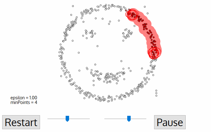
DBSCAN Smiley Face Clustering

1. 1. DBSCAN begins with an arbitrary starting data point that has not been visited. The neighborhood of this point is extracted using a distance epsilon ε (All points which are within the ε distance are neighborhood points).
   2. If there are a sufficient number of points (according to minPoints) within this neighborhood then the clustering process starts and the current data point becomes the first point in the new cluster. Otherwise, the point will be labeled as noise (later this noisy point might become the part of the cluster). In both cases that point is marked as “visited”.
   3. For this first point in the new cluster, the points within its ε distance neighborhood also become part of the same cluster. This procedure of making all points in the ε neighborhood belong to the same cluster is then repeated for all of the new points that have been just added to the cluster group.
   4. This process of steps 2 and 3 is repeated until all points in the cluster are determined i.e all points within the ε neighborhood of the cluster have been visited and labelled.
   5. Once we’re done with the current cluster, a new unvisited point is retrieved and processed, leading to the discovery of a further cluster or noise. This process repeats until all points are marked as visited. Since at the end of this all points have been visited, each point well have been marked as either belonging to a cluster or being noise.

DBSCAN poses some great advantages over other clustering algorithms. Firstly, it does not require a pe-set number of clusters at all. It also identifies outliers as noises unlike mean-shift which simply throws them into a cluster even if the data point is very different. Additionally, it is able to find arbitrarily sized and arbitrarily shaped clusters quite well.

The main drawback of DBSCAN is that it doesn’t perform as well as others when the clusters are of varying density. This is because the setting of the distance threshold ε and minPoints for identifying the neighborhood points will vary from cluster to cluster when the density varies. This drawback also occurs with very high-dimensional data since again the distance threshold ε becomes challenging to estimate.

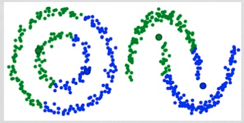
Expectation–Maximization (EM) Clustering using Gaussian Mixture Models (GMM)

One of the major drawbacks of K-Means is its naive use of the mean value for the cluster center. We can see why this isn’t the best way of doing things by looking at the image below. On the left hand side it looks quite obvious to the human eye that there are two circular clusters with different radius’ centered at the same mean. K-Means can’t handle this because the mean values of the clusters are a very close together. K-Means also fails in cases where the clusters are not circular, again as a result of using the mean as cluster center.

Two failure cases for K-Means

Gaussian Mixture Models (GMMs) give us more flexibility than K-Means. With GMMs we assume that the data points are Gaussian distributed; this is a less restrictive assumption than saying they are circular by using the mean. That way, we have two parameters to describe the shape of the clusters: the mean and the standard deviation! Taking an example in two dimensions, this means that the clusters can take any kind of elliptical shape (since we have standard deviation in both the x and y directions). Thus, each Gaussian distribution is assigned to a single cluster.

In order to find the parameters of the Gaussian for each cluster (e.g the mean and standard deviation) we will use an optimization algorithm called Expectation–Maximization (EM). Take a look at the graphic below as an illustration of the Gaussians being fitted to the clusters. Then we can proceed on to the process of Expectation–Maximization clustering using GMMs.

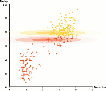
EM Clustering using GMMs

1. 1. We begin by selecting the number of clusters (like K-Means does) and randomly initializing the Gaussian distribution parameters for each cluster. One can try to provide a good guesstimate for the initial parameters by taking a quick look at the data too. Though note, as can be seen in the graphic above, this isn’t 100% necessary as the Gaussians start our as very poor but are quickly optimized.
   2. Given these Gaussian distributions for each cluster, compute the probability that each data point belongs to a particular cluster. The closer a point is to the Gaussian’s center, the more likely it belongs to that cluster. This should make intuitive sense since with a Gaussian distribution we are assuming that most of the data lies closer to the center of the cluster.
   3. Based on these probabilities, we compute a new set of parameters for the Gaussian distributions such that we maximize the probabilities of data points within the clusters. We compute these new parameters using a weighted sum of the data point positions, where the weights are the probabilities of the data point belonging in that particular cluster. To explain this in a visual manner we can take a look at the graphic above, in particular the yellow cluster as an example. The distribution starts off randomly on the first iteration, but we can see that most of the yellow points are to the right of that distribution. When we compute a sum weighted by the probabilities, even though there are some points near the center, most of them are on the right. Thus naturally the distribution’s mean is shifted closer to those set of points. We can also see that most of the points are “top-right to bottom-left”. Therefore the standard deviation changes to create an ellipse that is more fitted to these points, in order to maximize the sum weighted by the probabilities.
   4. Steps 2 and 3 are repeated iteratively until convergence, where the distributions don’t change much from iteration to iteration.

There are really 2 key advantages to using GMMs. Firstly GMMs are a lot more flexible in terms of cluster covariance than K-Means; due to the standard deviation parameter, the clusters can take on any ellipse shape, rather than being restricted to circles. K-Means is actually a special case of GMM in which each cluster’s covariance along all dimensions approaches 0. Secondly, since GMMs use probabilities, they can have multiple clusters per data point. So if a data point is in the middle of two overlapping clusters, we can simply define its class by saying it belongs X-percent to class 1 and Y-percent to class 2. I.e GMMs support mixed membership.

Agglomerative Hierarchical Clustering

Hierarchical clustering algorithms actually fall into 2 categories: top-down or bottom-up. Bottom-up algorithms treat each data point as a single cluster at the outset and then successively merge (or agglomerate) pairs of clusters until all clusters have been merged into a single cluster that contains all data points. Bottom-up hierarchical clustering is therefore called hierarchical agglomerative clustering or HAC. This hierarchy of clusters is represented as a tree (or dendrogram). The root of the tree is the unique cluster that gathers all the samples, the leaves being the clusters with only one sample. Check out the graphic below for an illustration before moving on to the algorithm steps

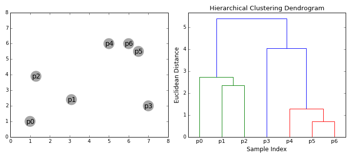
Agglomerative Hierarchical Clustering

1. 1. We begin by treating each data point as a single cluster i.e if there are X data points in our dataset then we have X clusters. We then select a distance metric that measures the distance between two clusters. As an example we will use average linkage which defines the distance between two clusters to be the average distance between data points in the first cluster and data points in the second cluster.
   2. On each iteration we combine two clusters into one. The two clusters to be combined are selected as those with the smallest average linkage. I.e according to our selected distance metric, these two clusters have the smallest distance between each other and therefore are the most similar and should be combined.
   3. Step 2 is repeated until we reach the root of the tree i.e we only have one cluster which contains all data points. In this way we can select how many clusters we want in the end, simply by choosing when to stop combining the clusters i.e when we stop building the tree!

Hierarchical clustering does not require us to specify the number of clusters and we can even select which number of clusters looks best since we are building a tree. Additionally, the algorithm is not sensitive to the choice of distance metric; all of them tend to work equally well whereas with other clustering algorithms, the choice of distance metric is critical. A particularly good use case of hierarchical clustering methods is when the underlying data has a hierarchical structure and you want to recover the hierarchy; other clustering algorithms can’t do this. These advantages of hierarchical clustering come at the cost of lower efficiency, as it has a time complexity of O(n³), unlike the linear complexity of K-Means and GMM.

Conclusion

There are your top 5 clustering algorithms that a data scientist should know! We’ll end off with an awesome visualization of how well these algorithms and a few others perform, courtesy of Scikit Learn!